Batch Inference at Scale: How to Maximize GPU Utilization

This post walks through a sample architecture for running 100M+ LLM inference calls with near-maximal GPU utilization on Union using Flyte’s orchestration primitives.

GPUs are brutally expensive to idle. And yet, that’s what most batch inference pipelines do: load a model, process some data, hit a straggler, wait, eventually finish. If you’re running evals at scale, generating synthetic datasets, scoring large corpora or doing multi-round LLM judging, you’ve probably already felt the cost of this the hard way.

The core problem isn’t that inference is slow. It’s that the orchestration around inference is naive. Data gets materialized into memory all at once. Workers finish at different rates and sit idle waiting for each other. Stragglers block entire rounds. Models load and unload repeatedly on every task invocation. All of this is infrastructure overhead eating into what should be GPU compute time.

The architecture in this post solves each of these problems directly. It’s built on Flyte, runs on Union, and gives you two concrete dispatch strategies depending on the shape of your workload. By the end you’ll understand not just how it works, but why the design choices were made, and how to tune it for your own pipeline.

Why naive batch inference falls apart

Before we get into the architecture, let’s be precise about what goes wrong with the obvious approach. The obvious approach looks like this: take your dataset, split it into chunks, spin up workers, run inference, collect results. Four things break when you take this to scale.

Memory pressure from materializing the dataset: If you load 100M samples upfront, you’re allocating gigabytes of data into memory before a single inference call has happened. Even with distributed storage, the overhead is real and entirely avoidable.

GPU waste from uneven workloads: LLM inference isn’t uniform as some prompts are longer and some outputs trigger more decoding steps. When one worker is stuck on a difficult batch, every other worker either waits or drains its work queue and idles.

The straggler problem: In any multi-round judging or approval pipeline, some samples get rejected and need another pass. If your architecture doesn’t handle stragglers gracefully, a handful of slow samples can hold the entire pipeline hostage, blocking the round from closing while GPUs sit mostly unused.

Cold start overhead: Loading a large model onto a GPU takes time. A 70B model at fp16 is roughly 140 GB, so it does not fit on a single 80 GB card; loading it across two A100-80GBs with tensor parallelism takes minutes. Even a 13B model that fits on one card costs 30–60 seconds on fast NVMe. In a naive architecture, every new pod pays this cost upfront. If you’re spinning up hundreds of pods, that’s a lot of model loading that never touches a single real sample.

The architecture we’re looking at fixes all four. Let’s go through the primitives it’s built on, then the design itself.

The platform: Flyte on Union

Flyte and Union together give you four primitives that do most of the heavy lifting in this architecture. Worth understanding each one clearly, because they solve different problems at different layers.

`JsonlDir` as a streaming primitive: The `JsonlDir` type ships in a separate plugin (`pip install flyteplugins-jsonl`, then from `flyteplugins.jsonl import JsonlDir, JsonlFile`). It lets you work with JSONL data stored in object storage (S3, GCS) without loading it all into memory. The dataset is split into shards, each shard is streamed record by record, and the memory footprint stays constant whether you are processing 1M samples or 100M. More on how this works under the hood in the next section.

Reusable containers: By default, every task execution in Flyte spins up a fresh container and discards it when done. For batch inference that’s a problem. Reusable containers fix this by maintaining a persistent pool via `ReusePolicy`. The model loads once and stays hot. Two timeouts matter. `idle_ttl` (default 30 s) shuts down the whole environment once it has been idle that long, so it needs to exceed the gap between rounds: set it too short and you’re cold-starting containers mid-pipeline, too long and you’re paying for idle GPU time at the tail end of a run. `scaledown_ttl` (default 30 s) is the minimum time an individual idle replica waits before removal, which damps churn when work arrives in bursts.

Dynamic batchers: This operates inside each container, at inference time, and is a separate concern from container lifecycle entirely. When multiple concurrent tasks are submitting samples asynchronously, the dynamic batcher accumulates those individual submissions and groups them into batched model calls before they hit the GPU. A single forward pass over 256 samples is far cheaper than 256 individual forward passes. The container handles scheduling; the batcher handles GPU utilization within that container.

Replica-level parallelism: Tasks run with multiple replicas, which is effectively a pool of identical GPU workers. Combined with the `concurrency` setting on reusable containers, this is what determines how many shards the system processes in parallel. At most `replicas × concurrency` shards are in flight at once.

JsonlDir and backpressure

`JsonlDir` is worth spending time on because it’s doing more work than it looks like at first glance.

At the surface level, it’s a directory of JSONL shard files stored in object storage: `part-00000.jsonl`, `part-00001.jsonl` and so on. Tasks read from it by iterating shards in sorted order. Two things about it matter for what follows: how reads stay bounded, and how writes rotate.

Reads stream, they never materialize

`iter_records()` is an async generator over `readline()`, with 64 KB chunked decompression for `.jsonl.zst`. A task reading a 20,000-record shard holds one record at a time, not 20,000. Memory is bounded by what you choose to accumulate rather than by shard size, which is why the tasks below batch in 2,000-record chunks and nothing larger ever exists.

Backpressure

Without backpressure, a reader racing ahead of a slow GPU produces memory bloat: you buffer records you cannot process yet. This architecture takes its backpressure from the dispatcher rather than the reader. The driver caps how many shards are in flight, so the loop that dispatches them stalls whenever the GPU pool is saturated. The consumer signals the producer to slow down without any explicit coordination code, and the GPU stays the bottleneck. That is exactly what you want.

You will see this mechanism in `_dispatch_bounded` below.

Automatic shard rotation on writes

`JsonlDir` also handles the write side. When your inference task writes results, `JsonlDir` manages shard rotation automatically, splitting output into new shard files when a shard hits a configurable size limit (default: 256 MB uncompressed). You don’t manage file handles or shard indices. You just write records.

from flyteplugins.jsonl import JsonlDir  # pip install flyteplugins-jsonl

async with JsonlDir.new_remote("results").writer(max_records_per_shard=20_000) as w:
    for result in results:
        await w.write(result)
# Shards rotate at 20,000 records or 256 MB, whichever comes first.
# Output lands in object storage; you never manage file handles or shard indices.

Per-shard zstd compression is supported through the `.jsonl.zst` extension. On a 100M-sample dataset at roughly 1 KB per record, that is the difference between about 100 GB and about 25 GB in storage.

DynamicBatcher and TokenBatcher

The batching layer is where most of the GPU efficiency actually lives.

How DynamicBatcher works

The batcher acts as an accumulator between your async inference coroutines and the model. Coroutines submit individual samples via `await batcher.submit(record)`, which returns a `Future` as soon as the record is queued and suspends only when the submission queue is full, and the batcher groups them into optimally-sized batches before sending to the model.

The batcher accumulates across all concurrent tasks in the container, not just one. With 10-way concurrency, you have 10 tasks all submitting samples simultaneously. The batcher sees submissions from all of them, groups them together, and dispatches in cost-budgeted batches. That’s how you get high GPU utilization even when individual tasks are processing unevenly-sized shards. This works because all `concurrency` tasks in a reusable container share a single event loop. `DynamicBatcher` creates each record’s `Future` on the loop that called `submit()` and resolves it from its own processing loop, so every producer has to live on that same loop.

Three signals control when a batch gets dispatched:

1. Cost budget: The aggregator accumulates records until the running cost reaches `target_batch_cost`, then dispatches. The record that crosses the threshold is admitted in full, so a dispatched batch can exceed the budget by up to the cost of one record, and a single record larger than the budget forms an oversized batch on its own. Size your GPU headroom accordingly.
2. Hard cap: `max_batch_size` sets an absolute ceiling on records per batch regardless of cost.
3. Timeout: `batch_timeout_s` bounds the fill window, measured from the moment the batch’s first record is dequeued. When it expires the batcher dispatches whatever has accumulated, even a partial batch. This prevents stalls when arrival rates aren’t perfectly steady.

import asyncio
from flyte.extras import DynamicBatcher


async def process(batch: list[dict]) -> list[str]:
    """Your batch processing function.
    Must return results in the same order as input.

    Never block the event loop here. The aggregation loop and every producer
    coroutine share it, so a synchronous call stalls the whole batcher.
    """
    return await asyncio.to_thread(heavy_computation_batch, batch)

async with DynamicBatcher(
    process_fn=process,
    target_batch_cost=1000,   # stop filling once accumulated cost reaches this;
                              # the record that crosses it is admitted in full,
                              # so a batch can exceed the budget by one record
    max_batch_size=64,        # hard cap on records per batch
    min_batch_size=1,         # leave at 1: larger values re-queue undersized
                              # batches at the tail, reordering them
    batch_timeout_s=0.05,     # bounds the fill window, measured from the
                              # batch's first record
    prefetch_batches=2,       # batches pre-assembled ahead of the model;
                              # raise this if the processing loop starves
    max_queue_size=5_000,     # submission queue depth for backpressure,
                              # not a batching knob
) as batcher:
    # submit() returns a Future as soon as the record is queued, and suspends
    # only when the queue is full. That suspension is the backpressure.
    futures = [await batcher.submit(r, estimated_cost=10) for r in my_records]
    results = await asyncio.gather(*futures)

Cost estimation

The batcher uses cost estimates to decide how many records to group into each batch. You can provide them in several ways, checked in order:

1. Explicit: pass `estimated_cost` to `submit()`
2. Estimator function: pass `cost_estimator` to the constructor
3. Protocol: implement `estimate_cost()` on your record type
4. Default: falls back to `default_cost` (default: `1`)

TokenBatcher for LLM inference

For LLM workloads, `TokenBatcher` is a convenience subclass that uses token-aware parameter names and checks the `TokenEstimator` protocol.

This matters because LLM inference cost scales with the token count of a batch, not its record count. `DynamicBatcher` with a count-based cost caps records per batch, which forces you to size `max_batch_size` for your worst-case prompt: set it to 256 and a burst of 200-token prompts produces a 51,200-token batch that overruns a GPU provisioned for 12,800; set it to 64 to stay safe and a run of 50-token prompts dispatches at 3,200 tokens, a quarter of the budget. `TokenBatcher` inverts the constraint. It fills a token budget and lets the record count float, so 256 prompts at 50 tokens and 64 prompts at 200 tokens both dispatch as a single 12,800-token batch.

Neither batcher groups by sequence length. A long prompt arriving behind short ones lands in their batch, in arrival order. Whether that costs you anything is decided by `inference_fn`: if it builds one padded tensor per batch, the short prompts get padded up to the long one; if your serving stack packs sequences instead, length variation is free. Note that a token budget would not rescue you if it did pad. It bounds the sum of a batch's tokens, while a padded batch costs `n × max_len`.

import asyncio
from dataclasses import dataclass
from flyte.extras import TokenBatcher  # `Prompt` also ships here


@dataclass
class Prompt:
    text: str

    def estimate_tokens(self) -> int:
        """Rough token estimate (~4 chars per token)."""
        return len(self.text) // 4 + 1


def _generate(batch: list[Prompt]) -> list[str]:
    """Your model's batched entry point. Synchronous."""
    return model.generate([p.text for p in batch])


async def inference(batch: list[Prompt]) -> list[str]:
    # _generate is synchronous. Calling it inline would stall the event loop
    # that the aggregation loop and every producer coroutine live on.
    #
    # It must also never raise for a single bad element: the batcher sets any
    # exception it raises on every future in that batch.
    return await asyncio.to_thread(_generate, batch)


async with TokenBatcher(
    inference_fn=inference,
    target_batch_tokens=12_800,  # a stopping threshold, not a ceiling: leave
                                 # headroom for the record that crosses it
    max_batch_size=256,          # 256 x 50 tokens fills both at once
    batch_timeout_s=0.05,
    prefetch_batches=2,
    max_queue_size=5_000,
) as batcher:
    future = await batcher.submit(Prompt(text="What is 2+2?"))
    result = await future

`estimate_tokens` here counts prompt tokens only. If your budget is meant to bound GPU memory during generation, add the maximum number of tokens you intend to sample. The KV cache grows with every decode step and for long generations, the output dominates the prompt.

Monitoring utilization

The batcher exposes a `stats` property with real-time metrics:

stats = batcher.stats

# `utilization` measures the fraction of time process_fn is running. It says
# nothing about how full the batches were: a batcher fed one record at a time
# reports ~100% while every forward pass carries a single sample. Always read
# it alongside batch fullness.
print(f"Loop busy:      {stats.utilization:.1%}")
print(f"Avg batch size: {stats.avg_batch_size:.1f} / 256")       # max_batch_size
print(f"Avg batch cost: {stats.avg_batch_cost:.0f} / 12800")     # target_batch_tokens
print(f"Records done:   {stats.total_completed} in {stats.total_batches} batches")
print(f"Busy / idle:    {stats.busy_time_s:.1f}s / {stats.idle_time_s:.1f}s")

A healthy batcher shows two things at once: `utilization` above 0.9, meaning the processing loop is rarely waiting for work, and `avg_batch_cost` close to `target_batch_tokens`, meaning the batches it dispatches are actually full. Either number alone is misleading.

The levers, in the order worth trying. First, more concurrent producers: raise `concurrency` on the `ReusePolicy`, or submit more samples per task. This is almost always the real fix. Second, `prefetch_batches`, if the processing loop is starving between batches. Third, a longer `batch_timeout_s`, which trades tail latency for fuller batches.

Two things that look like levers and aren’t: `max_queue_size` bounds how far producers may run ahead before `submit()` suspends and nothing else. And a shorter `batch_timeout_s` makes batches smaller, which raises the reported utilization while lowering real throughput.

The data pipeline: streaming at scale

With those primitives in mind, here’s how the data flows through the system.

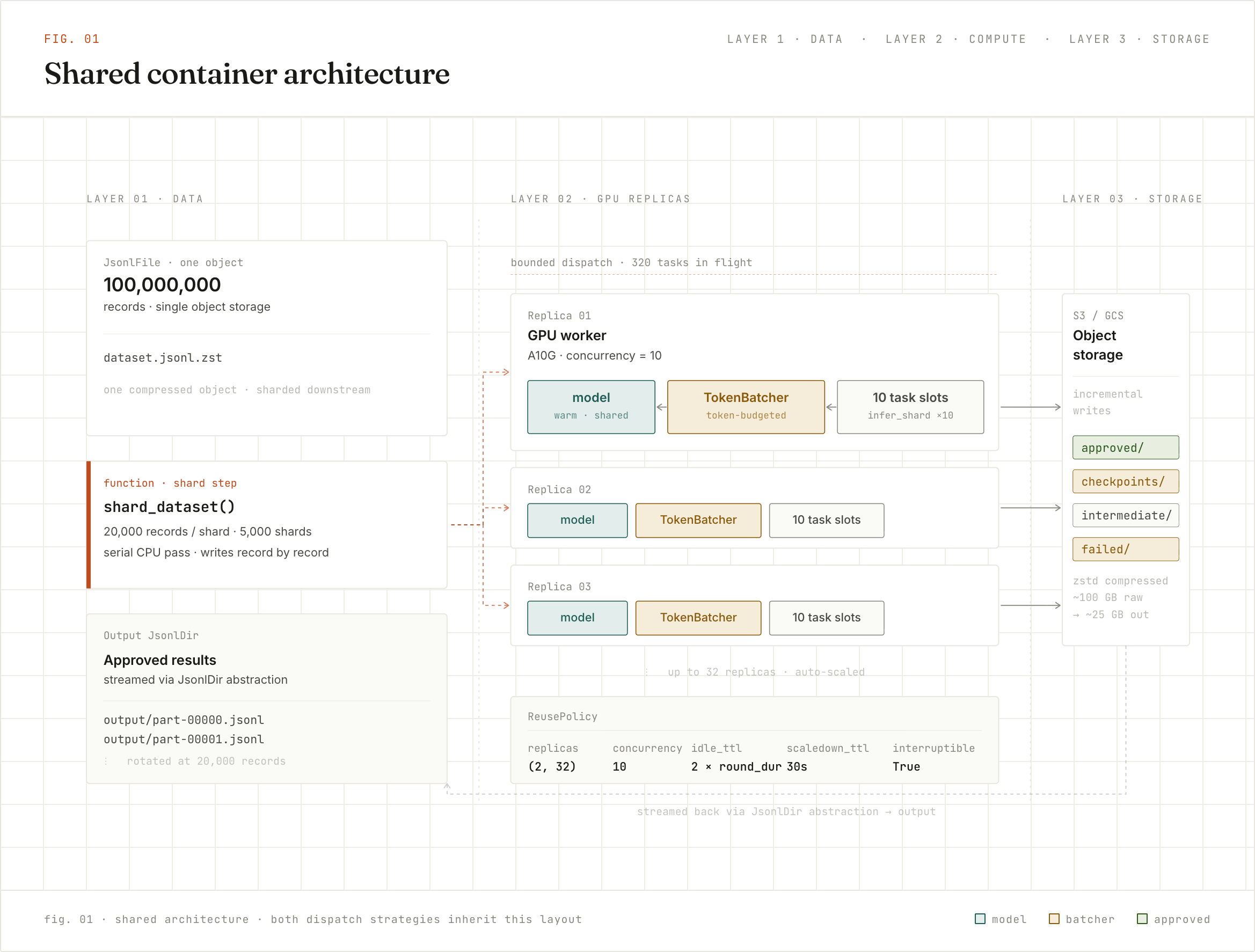
The example dataset is 100M samples stored as a `JsonlFile` in object storage. The first task converts it into a `JsonlDir`. A `JsonlFile` has no range or seek: `iter_records()` always starts at byte 0 and you cannot locate a JSONL line boundary without reading up to it. So 320 workers cannot each take a different slice of one file. Sharding is what turns an unsplittable object into N independently dispatchable units.

That first pass is serial, but it is a cheap one. It runs once, on a CPU node, before the GPU pool is needed, and every round afterwards reads the `JsonlDir`. Keep it off your GPU environment and never repeat it per round.

Because each shard becomes one task, shard size is a scheduling knob. Too large and each task runs for many minutes, so the final partial wave leaves most of the pool idle. Too small and you pay to list and open hundreds of thousands of objects. At 20,000 records per shard, 100M samples is 5,000 shards, and one task is a few minutes of work.

# Shard size trades scheduler overhead against the cost of the final wave.
@env.task   # the default CPU environment, not gpu_env: this pass needs no GPU
async def shard_dataset(src: JsonlFile) -> JsonlDir:
    """Turn one unsplittable file into N independently dispatchable shards."""
    out = JsonlDir.new_remote("sharded")
    async with out.writer(max_records_per_shard=20_000) as w:
        async for record in src.iter_records():
            await w.write(record)
    return out


data: JsonlDir = await shard_dataset(jsonl_file)
# Result: 5,000 shards of 20,000 records each, stored in object storage.

# Each shard becomes one task. Each task streams its shard through the
# batcher in 2,000-record chunks, so resident memory is one chunk, not one shard.

Flyte’s scheduler dispatches the shards across 32 replicas with 10-way concurrency per replica: 320 concurrent shard processors. At 5,000 shards / 320 concurrent workers, the dataset takes roughly 16 waves of scheduling.

The critical property: task inputs are references, not payloads. A task receives a shard handle and streams the records itself, so at any point in time only the chunk each worker is currently batching sits in memory. Everything else stays in object storage. Memory footprint is bounded by `active_workers × chunk_size`, not by dataset size and not by shard size.

import asyncio
from flyte.extras import TokenBatcher

_batcher: TokenBatcher | None = None
_batcher_loop: asyncio.AbstractEventLoop | None = None
_init_lock = asyncio.Lock()


async def get_batcher() -> TokenBatcher:
    """One batcher per container, shared by every concurrent task in it.

    DynamicBatcher creates each record's Future on the loop that called submit()
    and resolves it from its own processing loop, so all producers must share a
    single event loop with the batcher. That holds because the `concurrency`
    tasks in a reusable container run on one loop.
    """
    global _batcher, _batcher_loop
    loop = asyncio.get_running_loop()

    if _batcher is None:
        async with _init_lock:
            if _batcher is None:
                b = TokenBatcher(
                    inference_fn=inference,
                    target_batch_tokens=12_800,
                    max_batch_size=256,
                    batch_timeout_s=0.05,
                )
                await b.start()
                _batcher, _batcher_loop = b, loop

    if _batcher_loop is not loop:
        raise RuntimeError(
            "get_batcher() was called from a different event loop than the one "
            "that started the batcher; its futures would never resolve."
        )
    return _batcher

The two dispatch strategies

This is the core of the architecture. The system offers two fundamentally different approaches to dispatching work.

Strategy 1: re-dispatch remaining samples each round

Use this when approval rates are high and most samples complete within 1–3 rounds.

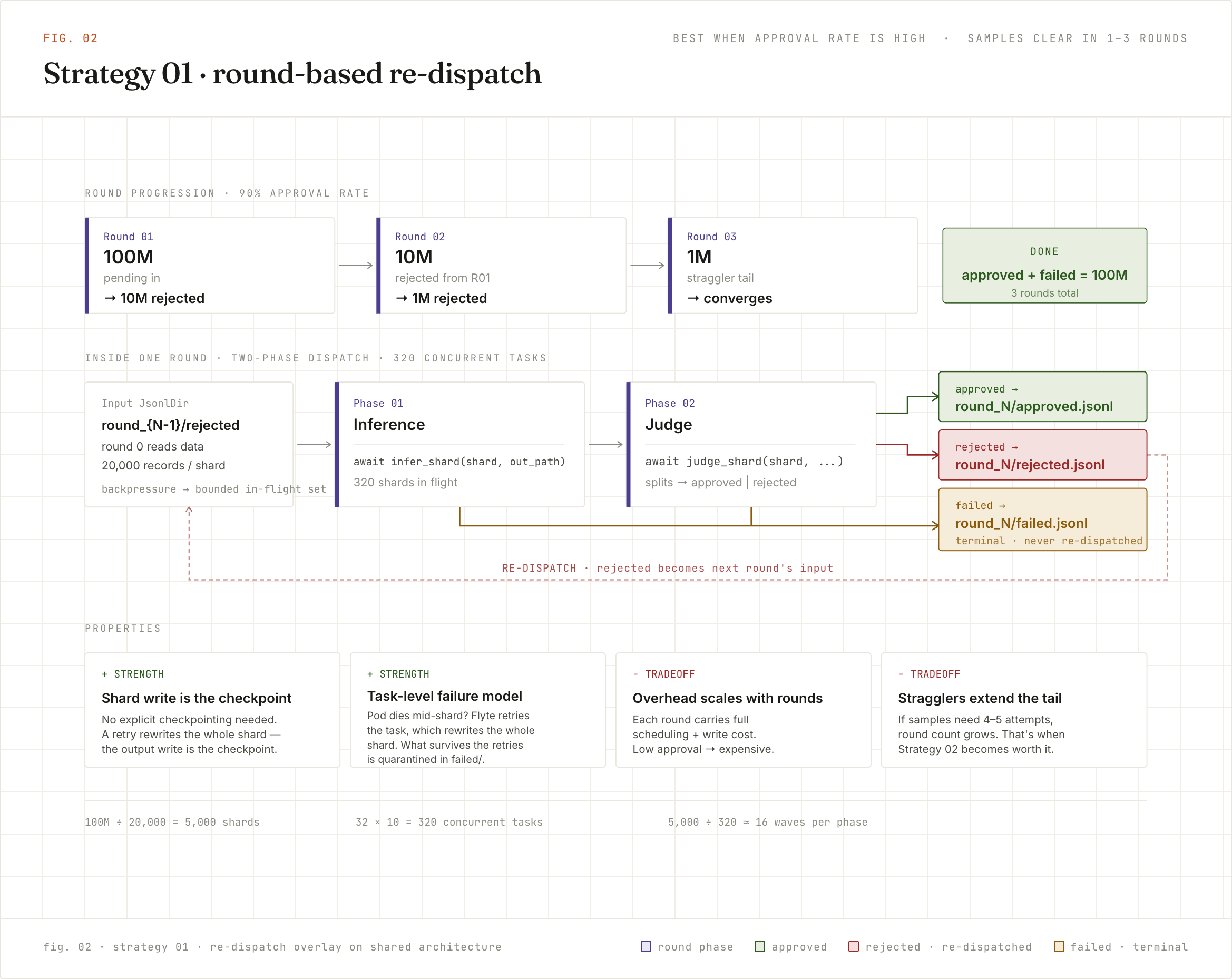
In this strategy, each round dispatches all pending samples together. After the round finishes, the workflow runs the judge, identifies which samples didn’t pass, and re-dispatches the remaining set as input to the next round.

Round 1: Infer 100M samples -> Judge -> Approved: 90M, Pending: 10M
Round 2: Re-dispatch 10M  -> Judge -> Approved: 9M,  Pending: 1M
Round 3: Re-dispatch 1M   -> Judge -> Done

Helpers like `build_infer_prompt`, `save_checkpoint` and `MAX_ROUNDS` are yours to supply; only the orchestration shape matters here. `get_batcher` is the exception, shown in full above, because the single-event-loop constraint it encodes is easy to get wrong.

The re-dispatch loop in the workflow:

import asyncio
import logging
from typing import Any

from flyteplugins.jsonl import JsonlDir, JsonlFile

logger = logging.getLogger(__name__)

MAX_IN_FLIGHT = 320     # 32 replicas × 10 concurrency
CHUNK_SIZE = 2_000      # records handed to the batcher at a time
SHARD_RECORDS = 20_000  # records per shard, and therefore per task

# Two one-liners, elided: _aiter() wraps a list as an async iterator, and
# _list_shards() walks a JsonlDir and returns its shards sorted by name.


async def _dispatch_bounded(source, task_fn, on_result, on_error=None, limit=MAX_IN_FLIGHT):
    """Dispatch task_fn over source, holding at most `limit` tasks in flight.

    Each outcome is delivered exactly once: to on_result on success, to on_error
    on failure. With on_error=None a failure propagates and stragglers are
    cancelled.
    """
    in_flight: dict[asyncio.Task, Any] = {}

    async def reap(when):
        done, _ = await asyncio.wait(in_flight.keys(), return_when=when)
        for t in done:
            item = in_flight.pop(t)
            exc = t.exception()          # does not raise; lets us branch
            if exc is None:
                await on_result(t.result())
            elif on_error is None:
                raise exc
            else:
                await on_error(item, exc)

    try:
        async for item in source:
            if len(in_flight) >= limit:
                await reap(asyncio.FIRST_COMPLETED)
            in_flight[asyncio.create_task(task_fn(item))] = item

        while in_flight:
            await reap(asyncio.FIRST_COMPLETED)
    finally:
        for t in in_flight:
            t.cancel()


@gpu_env.task(retries=3)
async def infer_shard(shard: JsonlFile, out_path: str) -> int:
    """Read one shard, infer, write one shard. Returns the record count.

    Input and output are references. Records never cross the task boundary,
    so resident memory is one CHUNK_SIZE chunk, not one shard.
    """
    batcher = await get_batcher()
    written = 0

    async def flush(chunk: list[dict], w) -> int:
        futures = [await batcher.submit(build_infer_prompt(r)) for r in chunk]
        # return_exceptions keeps one bad record from killing the shard. A bare
        # gather() re-raises, the task exhausts its retries, and the driver
        # quarantines all 20,000 records over a single malformed completion.
        results = await asyncio.gather(*futures, return_exceptions=True)
        ...  # write one row per record, each carrying a `status` of "ok" or "error"
        return len(chunk)

    async with JsonlFile(path=out_path).writer() as w:
        ...  # accumulate CHUNK_SIZE records from shard.iter_records(), then flush

    return written


@gpu_env.task(retries=3)
async def judge_shard(shard: JsonlFile, approved_path: str, rejected_path: str) -> dict[str, int]:
    """Split one inferred shard into an approved shard and a rejected shard.

    Same shape as infer_shard: stream, batch, gather with return_exceptions=True.
    A record whose inference failed skips the judge and goes straight to
    `rejected`, since "rejected" already means "needs another attempt" and
    MAX_ROUNDS is the backstop if it never converges.
    """
    ...  # returns {"approved": n, "rejected": m}


@env.task   # CPU: no GPU needed to repack shards
async def recompact(src: JsonlDir, name: str) -> JsonlDir:
    """Rewrite a JsonlDir into full shards.

    judge_shard emits one rejected shard per inferred shard, so the shard count
    survives every round while the record count collapses. Without this, a 90%
    approval rate leaves round 3 dispatching 5,000 tasks to handle 199 records
    each. The pass is serial, but it runs over a set an order of magnitude
    smaller than the round before it.
    """
    out = JsonlDir.new_remote(name)
    async with out.writer(max_records_per_shard=SHARD_RECORDS) as w:
        async for record in src.iter_records():
            await w.write(record)
    return out


@env.task
async def batch_inference_workflow(data: JsonlDir) -> JsonlDir:
    results = JsonlDir.new_remote("results")
    pending = data

    for round_num in range(MAX_ROUNDS):
        inferred = JsonlDir.new_remote(f"round_{round_num}/inferred")
        rejected = JsonlDir.new_remote(f"round_{round_num}/rejected")
        failed = JsonlDir.new_remote(f"round_{round_num}/failed")

        shards = await _list_shards(pending)
        if not shards:
            break

        totals = {"approved": 0, "rejected": 0}
        inferred_records = 0

        async def count_inferred(n: int) -> None:
            nonlocal inferred_records
            inferred_records += n

        async def do_infer(indexed):
            i, shard = indexed
            return await infer_shard(shard, f"{inferred.path}/part-{i:05d}.jsonl")

        async def do_judge(indexed):
            i, shard = indexed
            return await judge_shard(
                shard,
                f"{results.path}/round{round_num:02d}-part-{i:05d}.jsonl",
                f"{rejected.path}/part-{i:05d}.jsonl",
            )

        async def tally(counts):
            for status, n in counts.items():
                totals[status] += n

        async with failed.writer() as wf:

            def quarantine(phase):
                async def record(indexed, exc):
                    # Permanent, after Flyte retries are exhausted. Record it and
                    # move on. Never requeue: a deterministic failure would loop
                    # until MAX_ROUNDS, burning GPU on every pass.
                    await wf.write(
                        {"shard": indexed[1].path, "phase": phase, "error": repr(exc)}
                    )
                return record

            # Phase 1: inference. Each task writes its own output shard.
            await _dispatch_bounded(
                _aiter(list(enumerate(shards))), do_infer, count_inferred, quarantine("infer")
            )

            # Phase 2: judge. Approved records go straight into `results`; the
            # judge already holds them, so there is no copy pass.
            await _dispatch_bounded(
                _aiter(list(enumerate(await _list_shards(inferred)))),
                do_judge, tally, quarantine("judge"),
            )

        if totals["approved"] + totals["rejected"] != inferred_records:
            # A shard that exhausted its retries still left a partial output for
            # the judge to pick up. `failed` names the shard; this is how you
            # notice it happened at all.
            logger.warning("round %d: record count mismatch", round_num)

        if totals["rejected"] == 0:
            break

        # Rejected shards inherit their parent's shard count, so they shrink by
        # the approval rate every round. Repack before re-dispatching.
        pending = await recompact(rejected, f"round_{round_num}/pending")

    # If the loop exits on MAX_ROUNDS rather than convergence, the last round's
    # `rejected` dir holds every sample that never cleared. Inspect it; exhaustion
    # is not a normal completion path.
    return results

The `batch_inference_workflow` driver fans out across 32 replicas with 10-way concurrency, resulting in 320 shards in flight simultaneously. Each task receives a shard reference and reads the records itself; inside `infer_shard`, sample submissions flow into the batcher, which accumulates across all concurrent tasks in the container and dispatches to the model. The `judge_shard` phase works identically: the same fan-out, the same batcher, splitting records into `approved` and `rejected` shards. The rejected set becomes `pending` for the next round.

Why it works: On high-approval workloads, the pending set shrinks fast. Round 1 clears 90% of samples. Round 2 clears 90% of what’s left. By round 3 you’re dealing with a negligible tail. GPU utilization stays high because every round is a full fan-out, and the stragglers never accumulate enough to stall progress.

The tradeoff: If approval rates are low, this strategy amplifies costs. A pipeline with 50% approval per round leaves 50M samples pending after round 1, 25M after round 2. You’re doing significantly more total inference work, and each round carries the full overhead of scheduling, dispatching, writing intermediate results, and repacking the rejected set. That’s when you reach for Strategy 2.

Strategy 2: in-place retry inside the task

Use this when approval rates are low, samples frequently need multiple passes, and you want GPU utilization to stay high regardless of how many samples are churning.

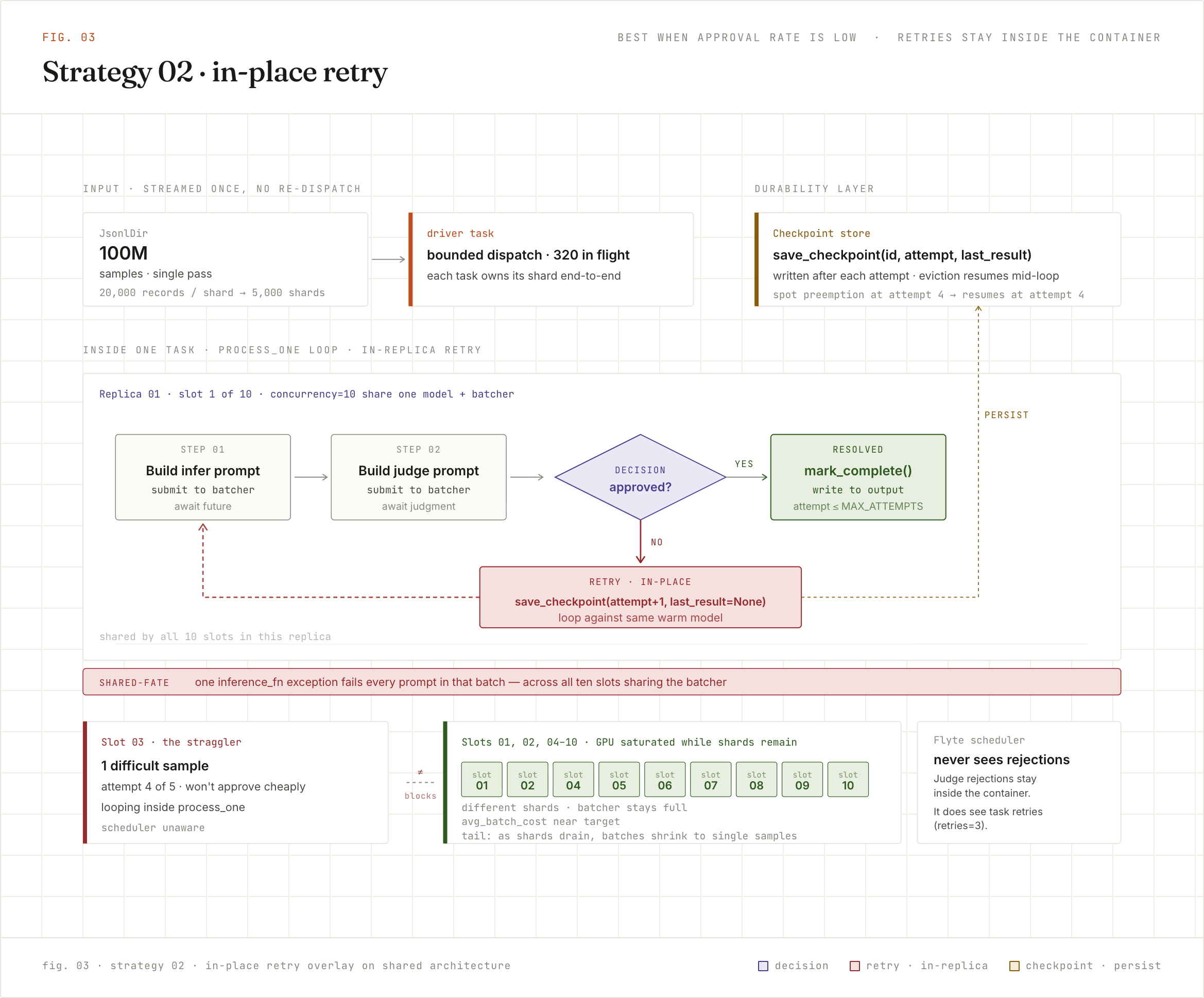
Both strategies use the same reusable container setup with 32 replicas, 10-way concurrency, where the model is loaded once and kept hot. What changes is where retry logic lives. In Strategy 1, a rejected sample exits the current round and gets re-queued into the next. The pod is done with it. In Strategy 2, the pod owns the sample until it’s approved or exhausted. Retry happens inside `process_one`, against the same warm model, without ever touching the scheduler.

@gpu_env.task(retries=3)
async def infer_shard_with_retry(shard: JsonlFile, out_path: str) -> dict[str, int]:
    """In-place retry. The pod owns each sample until it is approved or exhausted."""
    batcher = await get_batcher()
    counts = {"approved": 0, "max_attempts": 0, "error": 0}

    async def process_one(sample: dict) -> dict:
        try:
            state = await load_checkpoint(sample["id"])
            result = state.get("last_result")

            for attempt in range(state.get("attempt", 0), MAX_ATTEMPTS):
                if result is None:
                    future = await batcher.submit(build_infer_prompt(sample))
                    result = await future
                    await save_checkpoint(
                        sample["id"], attempt=attempt, last_result=result
                    )

                future = await batcher.submit(build_judge_prompt(sample, result))
                judgment = await future

                if judgment["approved"]:
                    await mark_complete(sample["id"])
                    return {**sample, "result": result,
                            "status": "approved", "attempts": attempt + 1}

                # Clear last_result explicitly. On resume we must re-infer, not
                # re-judge the output that was just rejected. Passing it here
                # is correct whether save_checkpoint merges or replaces.
                result = None
                await save_checkpoint(sample["id"], attempt=attempt + 1, last_result=None)

            return {**sample, "result": None,
                    "status": "max_attempts", "attempts": MAX_ATTEMPTS}
        except Exception as e:
            # Catches failures in this coroutine's own path: checkpoint I/O,
            # prompt building, a future that resolved to an exception.
            #
            # Mind the blast radius. If `inference_fn` itself raises, the batcher
            # sets that exception on every future in the batch, and that batch is
            # assembled across all ten concurrent tasks in the container. Keep
            # `inference_fn` total — catch per-element parse errors there and
            # encode them in the result — or one bad completion lands here for a
            # few hundred healthy samples from unrelated shards.
            return {**sample, "result": None, "status": "error", "error": str(e)}

    async with JsonlFile(path=out_path).writer() as w:

        async def flush(chunk: list[dict]) -> None:
            results = await asyncio.gather(*(process_one(s) for s in chunk))
            for r in results:
                counts[r["status"]] += 1
            await w.write_many(results)

        chunk: list[dict] = []
        async for record in shard.iter_records():
            chunk.append(record)
            if len(chunk) == CHUNK_SIZE:
                await flush(chunk)
                chunk = []
        if chunk:
            await flush(chunk)

    return counts

The checkpoint pattern is doing more work than it looks like. Each attempt writes its state before moving on. If the container goes down mid-attempt due to spot preemption or OOM, the next container picks up from the last saved state rather than starting over.

Compare that to Strategy 1, where you don’t need explicit checkpointing at all. The round structure gives you fault tolerance for free, but only because Flyte retries the failed task and the retried task rewrites its whole shard. That is the part worth being precise about: the next round’s input is `rejected`, not “everything that wasn’t approved”, so a shard whose records reach neither sink vanishes from the run. Flyte’s `retries=3` covers the transient case and the `failed` quarantine dir covers what survives it. With both in place the `JsonlDir` write pattern is your checkpoint and nothing extra is needed.

The two differ in the cost of recovery. Strategy 1’s recovery unit is the shard: a retried task re-infers all 20,000 records from scratch, because the output shard is its only checkpoint. Strategy 2 has no round boundary to fall back on, so `save_checkpoint` becomes the mechanism that makes in-place retry safe on interruptible infrastructure. Its recovery unit is the sample. An eviction at attempt 4 of 5 picks up at attempt 4, not attempt 0.

Then there’s the straggler behavior. Say 1,999 of 2,000 samples in a chunk approve on the first attempt. The one difficult sample keeps retrying inside `process_one`. The other 9 concurrency slots in the same container are working on entirely different shards, so a single retrying sample costs one slot rather than the whole container, and the GPU keeps receiving full batches from its neighbours. The caveat is the very end of a run: once most shards have drained, the remaining slots can all be occupied by single-sample retry loops, and batch sizes collapse. Strategy 2 makes the tail cheap but it does not make it free.

Why this works for low-approval workloads: In Strategy 1, a 50% approval rate means round 2 is scheduling 50M samples with full fan-out, scheduling overhead and intermediate writes. Strategy 2 handles those retries where they happen, inside the container, against a model that’s already warm. The scheduler never sees them. What you give up is simplicity. The code is more involved, the checkpoint infrastructure needs to exist and you need confidence that your retry loop eventually converges.

One more thing: always put a hard cap on `MAX_ROUNDS`. If you leave retries open-ended and your judge has a flaw, the pipeline can keep running indefinitely without it being immediately obvious. You usually only notice once the costs start adding up. And when the pipeline does hit the retry cap, that should be treated as something worth investigating, not as a normal completion path.

The capacity math stays the same across both strategies:

Replicas:            32
Concurrency:         10        (tasks per container)
Shard size:          20,000    (records per shard = records per task)
Chunk size:          2,000     (records submitted to the batcher at a time)
Max batch size:      256       (samples per model call)

Shards:              100,000,000 / 20,000  = 5,000
Tasks in flight:     32 × 10               = 320
Records resident:    320 × 2,000           = 640,000   (one chunk per worker)
Scheduling waves:    5,000 / 320           ≈ 16        (the partial final wave
                                                        idles ~2% of GPU time)
Model calls (run):   100,000,000 / 256     ≈ 390,625   (lower bound: a token
                                                        budget may cap a batch
                                                        below 256 samples)

The numbers are identical across both strategies. What changes is entirely where retry work happens: at the scheduler level or inside the container. That single decision shapes your fault tolerance model, your infrastructure requirements, and how gracefully the pipeline degrades when approval rates are low.

Choosing between the two strategies

The decision comes down to one number: your approval rate per round.

If most samples pass on the first or second attempt, above roughly 70% approval per round, Strategy 1 is the right call. The pending set shrinks fast, the round structure keeps things simple, and you get fault tolerance for free from the `JsonlDir` write pattern. The code is straightforward and the failure modes are easy to reason about.

If approval rates are low, or your judging criteria are strict enough that samples regularly need three, four or five attempts, Strategy 1 starts to break down. Every retry goes back through the scheduler, so the overhead keeps piling up and the tail latency only gets worse. That’s where Strategy 2 starts making a lot more sense. Retries happen inside the container itself against a model that’s already warm, without constantly bouncing back through the scheduler.

That fault tolerance story is also what makes spot instances viable here. Strategy 1 recovers via the round structure; Strategy 2 recovers via checkpointing. Either way, a preempted container picks up where it left off rather than starting over. With `interruptible=True`, Flyte reschedules a preempted task automatically. Note that this system-level rescheduling is a separate tier from the `retries` count on the task, which is what covers application failures like a model OOM; you want both. Spot discounts typically land around 60–70% off on-demand, though the figure varies by region and instance type.

The judge in both strategies doesn’t have to be an LLM either. Union's human-in-the-loop support lets you insert a human review gate at the round boundary. The workflow pauses after each inference phase, surfaces the pending samples for a human reviewer, and resumes once approvals come back. The `JsonlDir` round structure maps cleanly onto this: each round’s `rejected` set is exactly the queue of samples waiting for human judgment. You get the same fan-out and streaming behavior, with a human in the approval loop instead of, or alongside, an automated judge. This is useful when judging criteria are genuinely subjective or when you want human oversight on low-confidence outputs before they get re-queued.

There’s also a hybrid worth considering. Run Strategy 1 for the first round or two to clear the easy approvals cheaply, then switch to Strategy 2 for the stubborn tail. Both strategies read from and write to `JsonlDir`, so the output of one is a valid input to the other:

@env.task
async def hybrid_batch_inference(data: JsonlDir) -> JsonlDir:
    results = JsonlDir.new_remote("results")
    pending = data

    # Strategy 1: clear the easy approvals across a few rounds. `run_round` is the
    # loop body from batch_inference_workflow: it writes approved records straight
    # into `results` and returns the round's totals and its rejected shards.
    for round_num in range(STRATEGY_1_ROUNDS):
        totals, rejected = await run_round(round_num, pending, results)
        if totals["rejected"] == 0:
            return results
        pending = await recompact(rejected, f"round_{round_num}/pending")

    # Strategy 2: in-place retry for the stubborn tail. Its rows carry a `status`
    # field, so a downstream filter separates approved from max_attempts and error.
    async def do_retry(indexed):
        i, shard = indexed
        return await infer_shard_with_retry(
            shard, f"{results.path}/tail-part-{i:05d}.jsonl"
        )

    tail_totals = {"approved": 0, "max_attempts": 0, "error": 0}

    async def tally(counts):
        for status, n in counts.items():
            tail_totals[status] += n

    await _dispatch_bounded(
        _aiter(list(enumerate(await _list_shards(pending)))), do_retry, tally
    )
    return results

The crossover point is mostly a judgment call. A reasonable rule of thumb is to switch to Strategy 2 once the pending set stops shrinking meaningfully between rounds. At that point, the remaining samples are unlikely to clear cheaply no matter how many times you keep re-dispatching them.

Closing thoughts

Not every batch inference workload needs this level of complexity. If you’re processing a few million samples with a strong judge and relatively low retry rates, a simple fan-out approach is usually enough.

But once datasets get large, approval rates become unpredictable, and GPU costs start mattering, these decisions begin to compound quickly. Streaming instead of materializing keeps memory usage under control. Backpressure ensures the GPU stays the bottleneck instead of the scheduler. Reusable containers help avoid repeated cold starts. And the two dispatch strategies let you adapt to actual retry behavior instead of forcing one approach onto every workload.

The nice part is that most of these decisions are encapsulated in the primitives themselves. The pipeline code ends up expressing intent rather than infrastructure concerns, which is usually what good orchestration should feel like.